Softening Muon for Better Optimization in Certain Applications
Muon is a relatively new first-order optimization algorithm. It empirically works well for transformers. However, Muon produced worse results than Adam on a problem that I was working on. Muon had a margin over Adam initially, but it gradually lost its lead and eventually fell behind. I had some non-standard settings which I won’t explain in detail; the only thing worth noting is that it involved finetuning an Adam-pretrained ViT on a domain task. After some numerical investigation, I hypothesized that Muon’s nonselective scaling over all singular vectors might be problematic. There were already plenty of methods that attempted to address this problem, but none was to my satisfaction since I believe a useful method should:
- Be well motivated;
- Be conceptually clean;
- Incur almost no runtime overhead compared to plain Muon.
Hence I set off to design a new method called Soft Muon. It turned out to work out well for our application. It also seemed to be novel (this field is moving too fast, so I didn’t check very carefully). Facing zero paper publication pressure, I think an informal post is the best way to keep a note of Soft Muon.
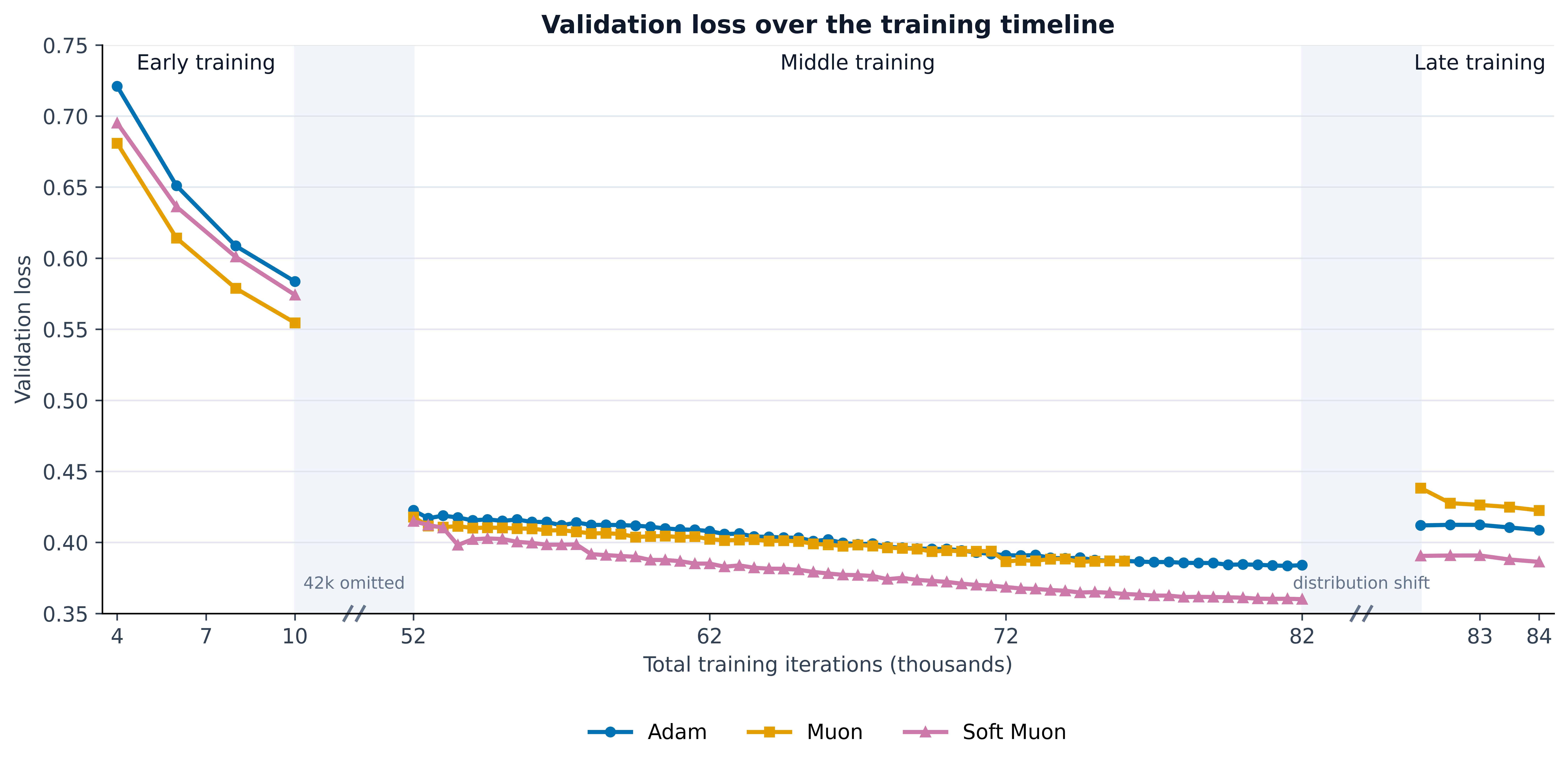
Below are the validation loss trajectories:
Background
Many gradient-based optimizers can be understood as choosing a steepest descent direction under a norm constraint. Given loss $L$ and gradient $G = \nabla_W L$, the update direction is $-v^*$, where
\[v^* = \arg\max_{\|v\| \le 1} \langle G, v \rangle\]For any norm $|\cdot|$, its dual norm is the value of the maximization problem
\[\|G\|_* := \max_{\|v\|\leq 1}\langle G,v\rangle,\]while the dual map defines the maximizer set:
\[\mathcal{D}(G) := \arg\max_{\|v\|\leq 1}\langle G,v\rangle.\]It’s established that the dual map is the same set as the subdifferential:
\[\mathcal{D}(G) = \partial\|G\|_*.\]For the nonzero inputs in the table below, assume also that every $\hat v_i$ is positive in the diagonal Mahalanobis case.
| Norm on $v$ | One dual-map output $v^*(G) \in \mathcal{D}(G)$ | Optimizer |
|---|---|---|
| $|v|_F$ (Frobenius) | $G / |G|_F$ | normalized SGD |
| $|v|_\infty$ (element-wise max) | $\mathrm{sign}(G)$ | signSGD |
| $\sqrt{\textstyle\sum_i v_i^2 \sqrt{\hat{v}_i}}$ (diag Mahalanobis) | $\dfrac{G_i / \sqrt{\hat{v}_i}}{\sqrt{\sum_j G_j^2 / \sqrt{\hat{v}_j}}}$ where $\hat{v}_i = \mathbb{E}[G_i^2]$ is the per-element second moment estimate |
normalized Adam-style direction |
| $|v|_\mathrm{op}$ (spectral/operator) | $UV^\top$ where $G = U\Sigma V^\top$ is the compact SVD over nonzero singular values |
Muon |
Motivating Muon
For a matrix parameter $W$, the operator norm is arguably a more natural update geometry than the Frobenius norm because it directly characterizes the largest change that $\Delta W$ can induce in a layer’s output. Specifically, for any layer input $x$, we have
\[\|(W + \Delta W)x - Wx\|_2 = \|\Delta W x\|_2 \leq \|\Delta W\|_\mathrm{op}\|x\|_2.\]Moreover, the operator norm is the tightest constant for which the above bound holds for arbitrary $x$. By comparison, the Frobenius norm cannot distinguish how the layer output’s change is distributed across singular directions.
For the spectral norm, the dual norm is the nuclear norm. If $G = U\Sigma V^\top$ is the compact SVD over its nonzero singular values, then
\[\|G\|_* = \sum_i \sigma_i, \qquad UV^\top \in \partial \|G\|_*.\]Thus the polar factor $UV^\top$ is a valid dual-map output. Choosing this output gives the idealized Muon update direction:
\[G_t = \nabla_{W_t}L = U_t\Sigma_tV_t^\top, \qquad W_{t+1} = W_t - \eta_t U_tV_t^\top.\]The polar map preserves the gradient’s singular vectors while replacing every nonzero singular value with 1. It therefore treats the weight update as a linear operator rather than as a collection of independent scalar updates. Practical Muon applies this map to momentum rather than directly to the raw gradient.
Some notes
Hard-ball vs soft-penalty. The dual-map formulation is a hard-ball constraint: the update has fixed norm regardless of gradient magnitude. For example, the Frobenius dual map gives gradient-normalized SGD ($G / |G|_F$), not vanilla SGD ($G$). Normalized SGD and idealized Muon are hard-ball methods. Standard convergence guarantees generally use learning rate decay; in stochastic settings, they typically require $\sum_t \eta_t = \infty$ and $\sum_t \eta_t^2 < \infty$. For a power-law schedule $\eta_t \asymp t^{-p}$, both requirements hold when $1/2 < p \leq 1$.
By contrast, vanilla SGD is a soft-penalty method: the update $-\eta G$ shrinks naturally as the gradient approaches zero, so it can converge even with a constant learning rate in deterministic settings (provided the loss landscape is well-behaved). The hard-ball formulation trades this natural convergence for better-conditioned updates, a worthwhile tradeoff when paired with an LR schedule.
Newton-Schulz approximation. Computing the full SVD every step is expensive and hard to parallelize. Muon approximates $UV^\top$ using 5 iterations of Newton-Schulz orthogonalization in bfloat16: each iteration uses three matmuls ($O(mn \cdot \min(m,n))$ per iteration, so $O(n^3)$ for square matrices). This is asymptotically more expensive than element-wise optimizers ($O(mn)$), but in practice the overhead is small (~2% of total training wall time in our run) because batched matmuls utilize the parallel computing resources of GPUs efficiently, and the matrices are small relative to the forward/backward pass.
From hard to soft orthogonalization
Let the momentum matrix at step $t$ be
\[M_t = \beta M_{t-1} + (1 - \beta) G_t\]Write its singular value decomposition as
\[M_t = U \operatorname{diag}(\sigma_1, \ldots, \sigma_r) V^\top, \qquad r = \min(m, n)\]Idealized Muon applies the hard polar map:
\[\sigma_i \mapsto 1 \qquad \text{for every nonzero } \sigma_i\]However, gradients can be noisy; not all singular directions of the momentum matrix are necessarily of equal importance. Thus we can use a soft gating function to modify the singular values:
\[\operatorname{gate}(\sigma_i) = \frac{\sigma_i}{\sqrt{\sigma_i^2 + \epsilon_t^2}}\]This has two useful limits:
\[\begin{aligned} \sigma_i \ll \epsilon_t &: & \operatorname{gate}(\sigma_i) &\approx \frac{\sigma_i}{\epsilon_t}, \\ \sigma_i \gg \epsilon_t &: & \operatorname{gate}(\sigma_i) &\approx 1. \end{aligned}\]Large singular directions therefore remain Muon-like, while weak directions can continue to stay weak instead of being lifted to unit.
From the gate to the matrix form. Consider one pair of right and left singular vectors, $v_i$ and $u_i$. By definition,
\[M_tv_i = \sigma_i u_i, \qquad M_t^\top M_tv_i = \sigma_i^2v_i.\]Thus $M_t^\top M_t + \epsilon_t^2I$ scales $v_i$ by $\sigma_i^2 + \epsilon_t^2$, and its inverse square root scales $v_i$ by the reciprocal square root:
\[\left(M_t^\top M_t + \epsilon_t^2I\right)^{-1/2} v_i = \frac{1}{\sqrt{\sigma_i^2 + \epsilon_t^2}}v_i.\]Multiplying by $M_t$ then gives
\[M_t\left(M_t^\top M_t + \epsilon_t^2I\right)^{-1/2}v_i = \frac{\sigma_i}{\sqrt{\sigma_i^2 + \epsilon_t^2}}u_i.\]This is exactly the desired gate on every singular direction; null-space directions remain zero. Therefore the matrix form is
\[\boxed{Q_t = M_t\left(M_t^\top M_t + \epsilon_t^2I\right)^{-1/2}}.\]Therefore, before the RMS correction introduced below, the corresponding update rule is
\[W_{t+1} = W_t - \eta_t Q_t = W_t - \eta_t M_t \left(M_t^\top M_t + \epsilon_t^2I\right)^{-1/2}.\]Choosing epsilon adaptively and efficiently
The remaining question is how to choose $\epsilon_t$. A fixed value makes little sense since it could be negligible for one momentum matrix and overwhelming for another. One reasonable proposal is to choose it relative to a typical singular value, such as their mean:
\[\bar{\sigma}(M_t) = \frac{1}{r}\sum_{i=1}^r \sigma_i, \qquad r = \min(m,n).\]Unfortunately, computing this mean requires an SVD at every optimizer step, which is too expensive for large-scale training. Instead, I use the RMS singular value as a convenient substitute:
\[\sqrt{\frac{1}{r}\sum_{i=1}^r\sigma_i^2} = \frac{\lVert M_t\rVert_F}{\sqrt{r}}.\]The right-hand side needs only a Frobenius norm, which is cheap to compute. Thus we can set
\[\epsilon_t = K\frac{\lVert M_t\rVert_F}{\sqrt{r}},\]where $K$ controls how aggressively weak singular directions are suppressed. I use $K=0.5$ for all matrices and training stages. In offline raw-gradient spectra, the RMS-to-mean ratio was $2.4$–$3.1$ for attention and $1.6$–$2.0$ for MLP. If the resulting gate values were applied as multiplicative filters to those raw singular values (i.e., $\sigma_i \leftarrow \sigma_i \operatorname{gate}(\sigma_i) = \sigma_i^2 / \sqrt{\sigma_i^2 + \epsilon_t^2}$), they would remove only $4.3$–$6.0\%$ and $7.9$–$10.8\%$ of the original Frobenius energy, respectively. These percentages indicate that the gate mainly affects weak directions; they are not energy removed from the final RMS-normalized Soft Muon update.
An efficient implementation reusing Muon primitives
Directly evaluating the inverse square root in $Q_t$ would require a new iterative solver. My implementation instead calls the same Newton-Schulz primitive as plain Muon.
The Muon primitive. For a full-row-rank wide matrix $X\in\mathbb{R}^{p\times q}$ with $p\leq q$, let
\[\operatorname{NS}(X) \approx (XX^\top)^{-1/2}X.\]For a rank-deficient $X$, the inverse square root is understood as the Moore–Penrose inverse square root. This is the polar factor of $X$. The implementation approximates it by first normalizing $X$ and then applying five matrix-multiplication-only Newton-Schulz iterations in bfloat16. Plain Muon obtains its update by calling this primitive on the momentum matrix.
Suppose $M_t\in\mathbb{R}^{m\times n}$ is wide (i.e., $m\leq n$); transpose it first if needed and transpose the result correspondingly.
Soft Muon as one augmented call. Append a scaled identity matrix:
\[A_t = \begin{bmatrix} M_t & \epsilon_t I_m \end{bmatrix}.\]First compute the matrix used by the Newton-Schulz primitive:
\[A_tA_t^\top = \begin{bmatrix}M_t & \epsilon_tI_m\end{bmatrix} \begin{bmatrix}M_t^\top \\ \epsilon_tI_m\end{bmatrix} = M_tM_t^\top + \epsilon_t^2I_m.\]Substitute this result and $A_t$ into the definition of $\operatorname{NS}(A_t)$:
\[\operatorname{NS}(A_t) = (M_tM_t^\top+\epsilon_t^2I_m)^{-1/2} \begin{bmatrix}M_t & \epsilon_tI_m\end{bmatrix}.\]The left multiplication acts on each horizontal block separately. Ignoring finite-iteration approximation error, the output is therefore
\[\operatorname{NS}(A_t) = \begin{bmatrix} \underbrace{(M_tM_t^\top+\epsilon_t^2I_m)^{-1/2}M_t}_{\text{first }n\text{ columns}} & \underbrace{\epsilon_t(M_tM_t^\top+\epsilon_t^2I_m)^{-1/2}}_{\text{last }m\text{ columns}} \end{bmatrix}.\]We keep the first $n$ columns. They are exactly the desired soft update:
\[Q_t = (M_tM_t^\top+\epsilon_t^2I_m)^{-1/2}M_t = M_t(M_t^\top M_t+\epsilon_t^2I_n)^{-1/2}.\]The two forms are equal because, under the SVD, both preserve the singular vectors and map each $\sigma_i$ to $\sigma_i/\sqrt{\sigma_i^2+\epsilon_t^2}$.
Thus Soft Muon needs one call to the existing Newton-Schulz primitive followed by a slice. The wider augmented matrix adds compute but requires no additional optimizer state.
The implementation makes one final correction to keep the step scale fixed as the spectrum changes.
Exact RMS restoration. For a full-row-rank wide matrix, exact plain Muon targets $m$ unit singular values and a Frobenius norm of $\sqrt m$. The soft output is therefore normalized to the same norm when it is nonzero:
\[\widehat Q_t = \begin{cases} \dfrac{\sqrt m}{\lVert Q_t\rVert_F}Q_t, & \lVert Q_t\rVert_F>0, \\ 0, & \lVert Q_t\rVert_F=0, \end{cases} \qquad \lVert\widehat Q_t\rVert_F= \begin{cases} \sqrt m, & \lVert Q_t\rVert_F>0, \\ 0, & \lVert Q_t\rVert_F=0. \end{cases}\]The implementation then reuses the AdamW-RMS-matched Muon multiplier proposed by in Muon is Scalable for LLM Training, namely $0.2\sqrt n$ for a wide $m\times n$ matrix:
\[\Delta W_t = -\eta_t\,0.2\sqrt n\,\widehat Q_t.\]Consequently, for a nonzero update,
\[\operatorname{RMS}(\Delta W_t) = \frac{\lVert\Delta W_t\rVert_F}{\sqrt{mn}} = 0.2\eta_t.\]The gate changes how a fixed update budget is distributed across singular directions without changing its total RMS.
The complete update for one momentum matrix can be summarized as
def soft_muon_update(W, M, learning_rate, K=0.5):
    """Apply one Soft Muon update to a 2D weight matrix.

    Args:
        W: Weight matrix being optimized.
        M: Momentum matrix for W at the current step; the same shape as W.
        learning_rate: Step size.
        K: Scale of epsilon relative to the RMS singular value.

    Returns:
        The updated weight matrix, with the same shape as W.
    """

    # Work in the wide orientation; transpose the result back afterward.
    transposed = M.rows > M.cols
    if transposed:
        M = M.T

    m, n = M.shape  # m <= n
    if frobenius_norm(M) == 0:
        return W
    epsilon = K * frobenius_norm(M) / sqrt(m)

    augmented = concat_columns(M, epsilon * identity(m))
    augmented_polar = muon_newton_schulz(augmented)
    Q = augmented_polar[:, :n]

    # Match the Frobenius norm and learning-rate scale of full-row-rank plain Muon.
    Q = Q * sqrt(m) / frobenius_norm(Q)
    update = 0.2 * sqrt(n) * Q

    if transposed:
        update = update.T
    return W - learning_rate * update
What happened in training
Three labels are used in the plots:
- Adam: the non-Muon optimizer control.
- Muon: standard orthogonalized momentum.
- Soft Muon: the method in this post, with $K=0.5$ and exact RMS restoration.
Loss
The trajectory at the beginning of this post shows the behavior that motivated the investigation. In the middle training phase, Muon’s lead over Adam shrank from about $0.0054$ to zero. Although Muon’s loss continued to improve, Adam caught up. In the final phase, after a data-distribution shift, Muon ended at $0.4226$ versus Adam’s $0.4087$.
Weight spectrum
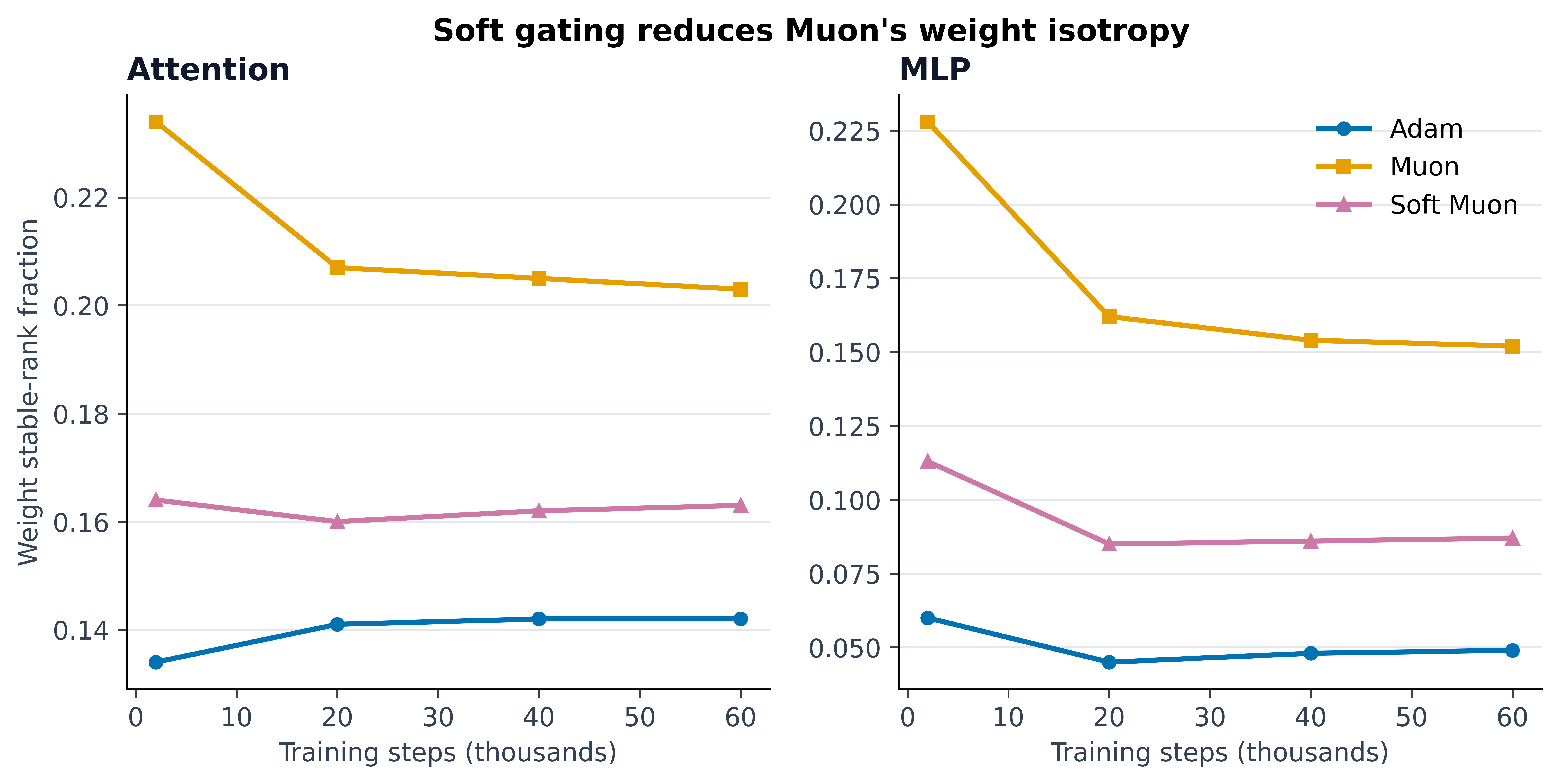
I measure weight isotropy using the normalized stable rank
\[\operatorname{stable\_rank\_fraction}(W) = \frac{\lVert W \rVert_F^2} {\sigma_{\max}(W)^2\min(m,n)}.\]A value near one means that the spectral energy is spread across many singular directions; a small value means that a few directions dominate. Muon produced much more isotropic weights than Adam. Soft Muon consistently sat between them, closing roughly $63$–$71\%$ of the stable-rank gap over training. Since all Muon variants had the same update RMS, this difference came from how the update budget was distributed, not from taking smaller steps.
The effect is cumulative: a moderate change to each update spectrum produced a large change in the final weight spectrum.
Gradient norm
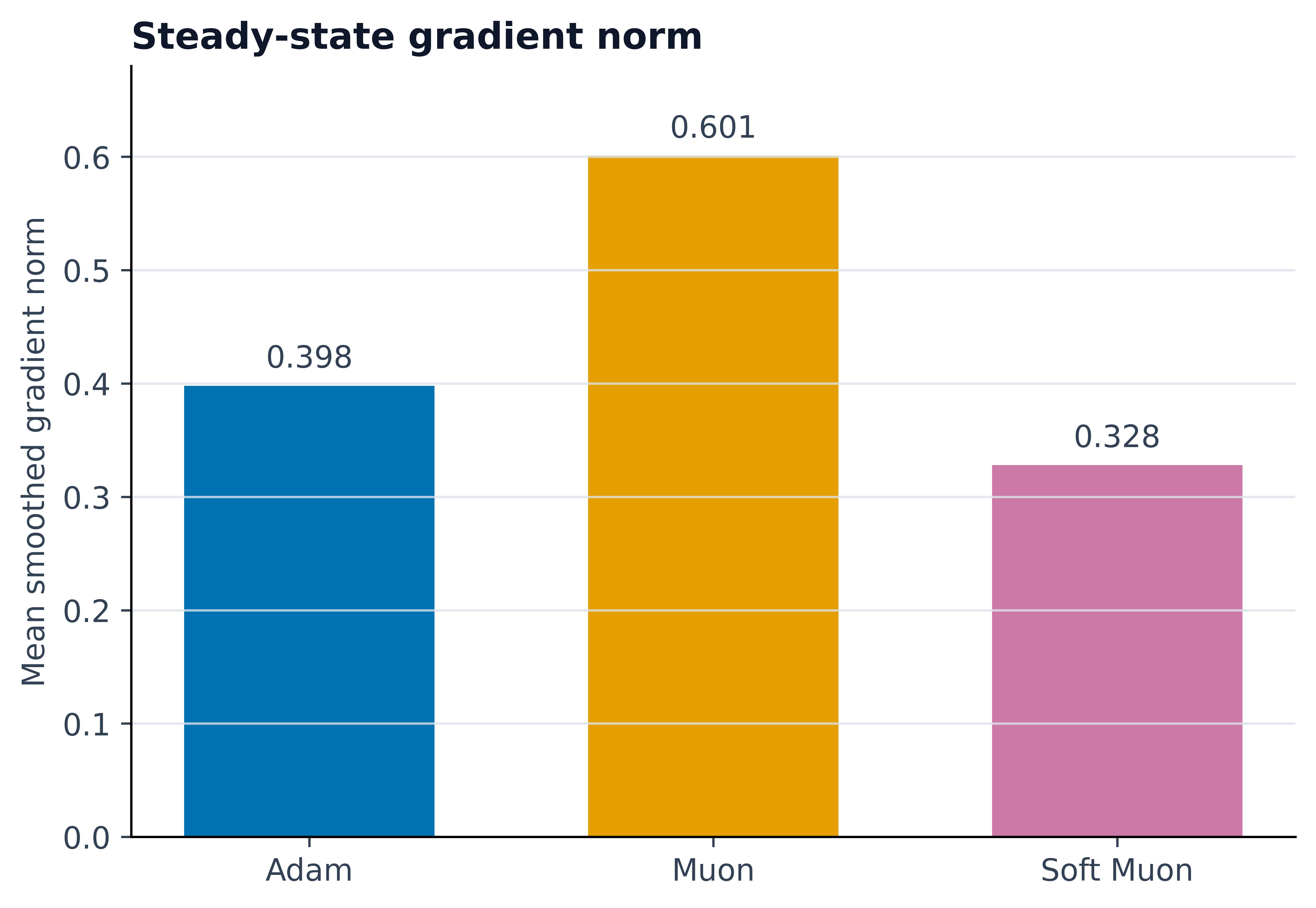
Over the final 10,000 steps, the mean smoothed raw gradient norm was $0.398$ for Adam, $0.601$ for Muon, and $0.328$ for Soft Muon. This gradient is measured before the optimizer transforms it, so the lower Soft Muon value is not a direct consequence of logging a gated update.
A smaller gradient at a comparable loss is consistent with a flatter local basin, but it is not enough by itself. I therefore also measured the weight spectrum and adversarial sharpness.
Adversarial sharpness
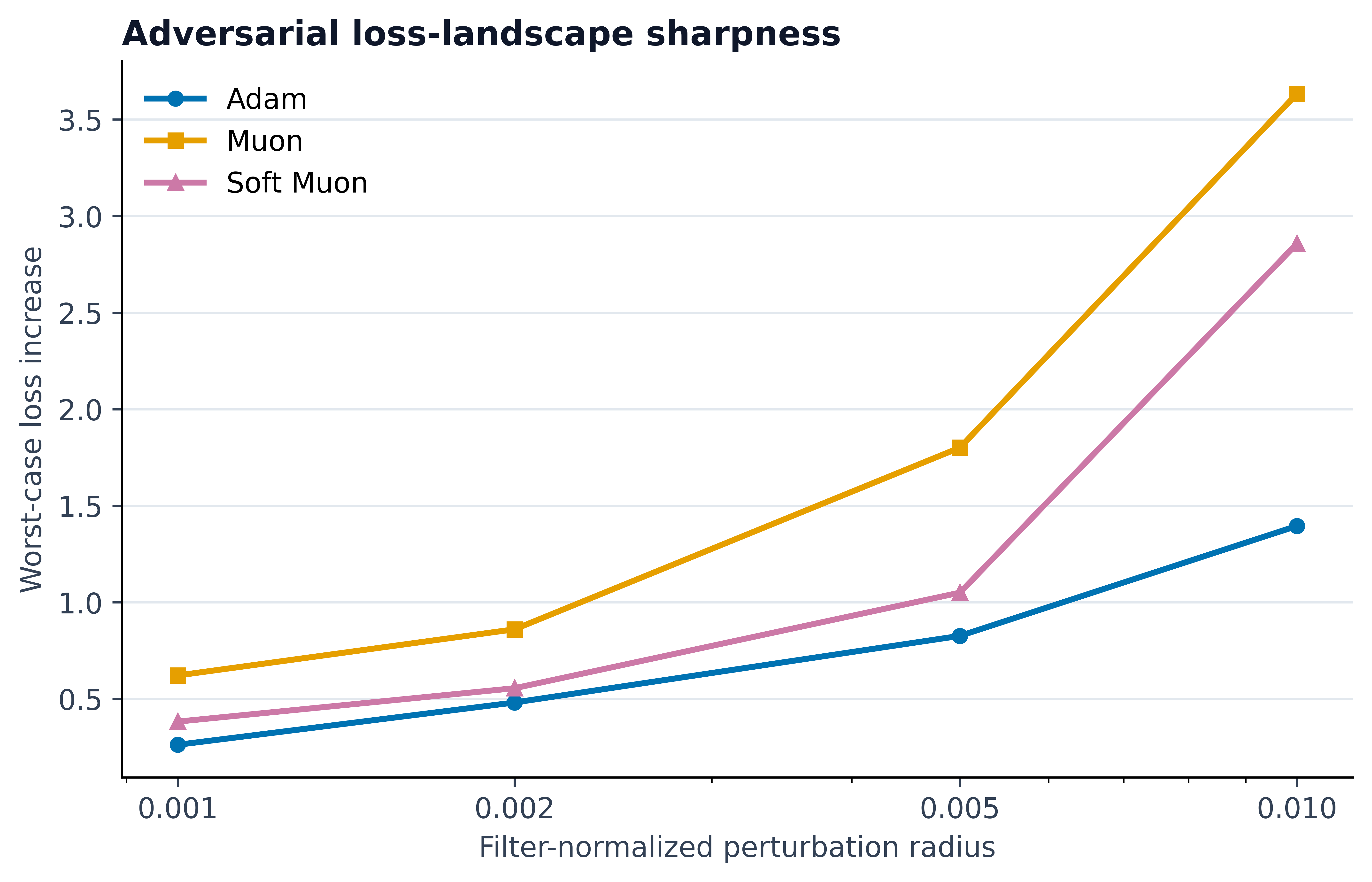
The sharpness probe perturbs the optimized matrix weights in a filter-normalized steepest-ascent direction and records the worst-case loss increase. Typically, less sharpness suggests better generalizability.
What is and is not new
The regularized polar map has appeared in several recent papers, some of which appeared after I did the experiments in May 2026. The methods differ mainly in how they choose the regularization scale and what problem they are trying to solve.
Move on Muon defines regularized Muon as
\[\operatorname{Orth}_\epsilon(M) = U\operatorname{diag}\left( \frac{\sigma_i}{\sqrt{\sigma_i^2+\epsilon^2}} \right)V^\top = \nabla_M\sum_i\left(\sqrt{\sigma_i^2+\epsilon^2}-\epsilon\right).\]Its focus is the smooth mirror-map and Hamiltonian interpretation of Muon. The analysis fixes $\epsilon>0$, and the experiments sweep absolute epsilon values. Adaptive choices of $\epsilon$ are left as future work.
Sharp Capacity Scaling of Spectral Optimizers in Learning Associative Memory uses the same map on the gradient,
\[G_t(G_t^\top G_t+\lambda_t^2I)^{-1/2}, \qquad \lambda_t\asymp \max\left\{ \frac{(\log d)^{2\alpha+2}}{d^\alpha}, \frac{(\log d)^2}{B} \right\}.\]Here the scale comes from a theoretical associative-memory model through the dimension $d$, frequency exponent $\alpha$, and batch size $B$.
Adaptive Matrix Online Learning through Smoothing studies the more general map
\[(SS^\top+LL^\top)^{-1/2}S, \qquad L_tL_t^\top=G^2I+\sum_{s\leq t}G_sG_s^\top.\]Setting $L=\epsilon I$ recovers the scalar regularized polar map, but the proposed algorithms use a history-dependent matrix smoother. Their goal is adaptive matrix online learning and nonsmooth nonconvex optimization under an operator-norm constraint.
SPECTRA wraps a base optimizer with soft spectral clipping,
\[H_{c_k}(X) =\left(I+\frac{XX^\top}{c_k^2}\right)^{-1/2}X =U\operatorname{diag}\left( \frac{c_k\sigma_i}{\sqrt{\sigma_i^2+c_k^2}} \right)V^\top.\]The factor $c_k$ gives an explicit spectral ceiling. During learning-rate warmup, SPECTRA uses
\[c_k=\frac{c\eta}{\eta_k}, \qquad \eta_kc_k=c\eta,\]so the effective update ceiling stays constant as $\eta_k$ changes; afterward it sets $c_k=c$. This is adaptation to the learning-rate schedule, not to the current matrix scale. SPECTRA uses the ceiling to constrain base-optimizer updates and, optionally, suppress large spectral spikes in raw gradients.
NorMuon and TrasMuon are relevant to the secondary calibration step rather than the core spectral map. NorMuon applies an EMA-based row adaptation after hard orthogonalization and then globally rescales the result. TrasMuon adds feature-wise damping after a similar calibration. Neither directly gates Muon’s singular values.
My focus is an efficient, scale-adaptive soft orthogonalization that can replace hard Muon in practical training:
\[\epsilon_t=K\frac{\lVert M_t\rVert_F}{\sqrt r}, \qquad Q_t=M_t(M_t^\top M_t+\epsilon_t^2I)^{-1/2}.\]This map is invariant to positive rescaling of $M_t$, requires no extra optimizer state, and can be evaluated by augmenting the matrix and reusing Muon’s Newton-Schulz primitive. The final RMS matching is an engineering control: it keeps the learning-rate scale fixed so the experiment isolates the effect of softening the spectrum. The practical question I wanted to answer was whether soft orthogonalization could change Muon’s learned geometry to achieve better loss for our application without requiring a separate solver. The experiments above suggest that it can.
Takeaway
Hard orthogonalization is an extreme spectral choice: every nonzero direction receives equal singular magnitude. A regularized polar map gives a continuous alternative. Setting its scale from the current momentum softens weak singular directions while leaving strong ones Muon-like. RMS matching is useful to match the Adam-tuned learning rate.
For our application, Soft Muon altered the final weight spectrum, reduced adversarial sharpness relative to standard Muon, and retained most of Muon’s initial validation-loss gain over Adam over the full training trajectory. The result supports a useful design principle: soften Muon’s weakest singular directions before spending a fixed update budget on them.
References
- Jordan et al., Muon: An Optimizer for Hidden Layers in Neural Networks, 2024.
- Liu et al., Muon is Scalable for LLM Training, 2025.
- Mustafi, Mukherjee, and Sriperumbudur, Move on Muon: A Hamiltonian Probability Gradient Flow Perspective of Muon Optimizer, 2026.
- Kim et al., Sharp Capacity Scaling of Spectral Optimizers in Learning Associative Memory, 2026.
- Jiang et al., Adaptive Matrix Online Learning through Smoothing with Guarantees for Nonsmooth Nonconvex Optimization, 2026.
- Jiang, Semenov, and Stich, Enhancing LLM Training via Spectral Clipping, 2026.
- Li et al., NorMuon: Making Muon More Efficient and Scalable, 2025.
- Cheng et al., TrasMuon: Trust-Region Adaptive Scaling for Orthogonalized Momentum Optimizers, 2026.